With Atom-JEPA, we showed that self-supervised pretraining in abstract representation space can produce state-of-the-art results on molecular ADMET and quantum-chemical property prediction tasks. One advantage of this approach is that it can learn from large molecular datasets without requiring labels. At the same time, previous approaches have shown that supervised pretraining can lead to strong downstream performance, even though the availability of labeled data limits its scale. This made us interested in combining the two: could adding a supervised objective in a second pretraining stage help build on the representations learned through Atom-JEPA’s self-supervised objectives?
To investigate this, we took our existing molecular Atom-JEPA model, pretrained on 19M molecules from the Uni-Mol dataset, and continued training with its original self-supervised objectives plus a supervised bioassay prediction objective. For this additional objective, we draw on Monroe, whose pretraining combines 81M PM6 molecules with quantum chemistry tasks alongside 1.5M PCBA molecules with roughly 1K bioassay tasks. Here, we start with just the bioassay component, using the same PCBA data to explore how this supervision complements Atom-JEPA’s self-supervised learning.
To evaluate the resulting model, Atom-JEPA-Bio, we use the same protocol as Pat Walters’ recent independent evaluation of Atom-JEPA. Atom-JEPA-Bio achieves best or statistically tied-for-best performance in 34 of 45 endpoint–metric combinations across the Biogen ADME and ExpansionRx datasets, compared with 18 of 45 for Monroe + TabPFN 3. On Biogen ADME, where Atom-JEPA previously trailed Monroe + TabPFN 3, Atom-JEPA-Bio now leads with 14 of 18 best-or-tied results versus 9 of 18. On ExpansionRx, it achieves 20 of 27 versus 9 of 27. Moreover, while the best results are still achieved with full finetuning, we also see exciting performance from frozen Atom-JEPA-Bio features paired with TabPFN 3, which perform on par with Monroe + TabPFN 3 on Biogen ADME without any encoder finetuning.
In this post, we present these results and walk through the method and implementation of the second pretraining stage, including how we combine the supervised and self-supervised objectives. We’ve updated the Atom-JEPA GitHub repository, and made Atom-JEPA-Bio available on Hugging Face and through the Atom-JEPA PyPI package for easy finetuning on new tasks.
Results
We evaluate Atom-JEPA-Bio with the protocol from Pat Walters’ Model Validation Central, which already includes the original Atom-JEPA. The protocol is the same for Biogen ADME and ExpansionRx. Each dataset has a fixed held-out test set. The remaining molecules are split into 5 cluster-grouped folds, and this is repeated 5 times with different shuffles, giving 25 train/validation splits. Each model trains on four folds, uses the fifth only to choose its best epoch, and is always scored on the same held-out test set. Methods are compared per endpoint and metric (MAE, Spearman ρ, R²) with Tukey’s HSD test at α = 0.05 over the 25 folds.
The study doesn’t publish its fold assignments, so we regenerated them with the study’s own splitting code and seed, and our training, validation and test set sizes match the reported ones on every fold. To check that the rest of the setup matches as well, we re-ran the original Atom-JEPA through the same pipeline and reproduced the study’s Biogen ADME results to within 0.005 on average across all endpoints and metrics. Atom-JEPA-Bio is finetuned with exactly the same recipe as Atom-JEPA in the study. The baseline results (LightGBM on Morgan fingerprints, ChemProp initialized from CheMeleon, Monroe + TabPFN 3, and Atom-JEPA) are taken from the study’s reported per-fold results rather than re-run by us.
TABLE 1
Compared models
| Model | Approach | Pretraining |
|---|---|---|
| Atom-JEPA-Bio FT | The same finetuning recipe as Atom-JEPA FT, starting from Atom-JEPA-Bio. | Atom-JEPA, then a second stage combining the Atom-JEPA objectives with bioassay supervision on ~1.5M PCBA molecules (~1K assays). |
| Atom-JEPA-Bio + TabPFN 3 | Frozen Atom-JEPA-Bio embeddings used as input features for TabPFN 3, with the same TabPFN 3 call as Monroe + TabPFN 3. | As Atom-JEPA-Bio FT. |
| Atom-JEPA FT | Atom-JEPA encoder finetuned multitask over all endpoints with a shared encoder and one head per endpoint, on 10 RDKit conformers per molecule; the test prediction is the mean over the 10 conformers. | Self-supervised Atom-JEPA on 19M Uni-Mol molecules. |
| Monroe + TabPFN 3 | Monroe’s frozen molecular embeddings used as input features for TabPFN 3, which predicts each endpoint in context from the training set. | ~81M PM6 molecules with 63 quantum-chemistry tasks, plus 1.56M PCBA molecules with ~1K bioassay tasks. |
| ChemProp + CheMeleon | Chemprop message-passing network (D-MPNN) on the 2D molecular graph, initialized from CheMeleon and finetuned multitask on related endpoints. | CheMeleon is pretrained to predict classical molecular descriptors. |
| LightGBM + Morgan | LightGBM gradient-boosted decision trees on Morgan count fingerprints, one model per endpoint. | None. |
Results for Atom-JEPA FT and the three baselines below the line are taken from the original Model Validation Central study’s reported per-fold results.
Biogen ADME
On the Biogen ADME dataset, Atom-JEPA-Bio improves on the original Atom-JEPA’s mean MAE across all six endpoints. The finetuned model achieves the lowest mean MAE on HLM, RLM, and HPPB, while frozen features paired with TabPFN 3 lead on SOL and RPPB. Monroe + TabPFN 3 remains strongest on MDR1_ER.
TABLE 2
Tukey HSD outcomes on Biogen ADME
| Model | Best alone | Tied for best | Worse | Best or tied |
|---|---|---|---|---|
| Atom-JEPA-Bio FT | 6 | 8 | 4 | 14 / 18 |
| Atom-JEPA-Bio + TabPFN 3 | 2 | 6 | 10 | 8 / 18 |
| Monroe + TabPFN 3 | 1 | 8 | 9 | 9 / 18 |
| Atom-JEPA FT | 0 | 0 | 18 | 0 / 18 |
| LightGBM + Morgan | 0 | 0 | 18 | 0 / 18 |
| ChemProp + CheMeleon | 0 | 0 | 18 | 0 / 18 |
Counted over 18 comparisons (6 endpoints × 3 metrics: MAE, Spearman ρ and R²), each over 25 cross-validation folds (5 × 5). Best alone: the best mean, significantly ahead of every other method. Tied for best: statistically indistinguishable from the best (α = 0.05). Worse: significantly worse than the best.
FIGURE 1
Test MAE on Biogen ADME with Tukey HSD intervals
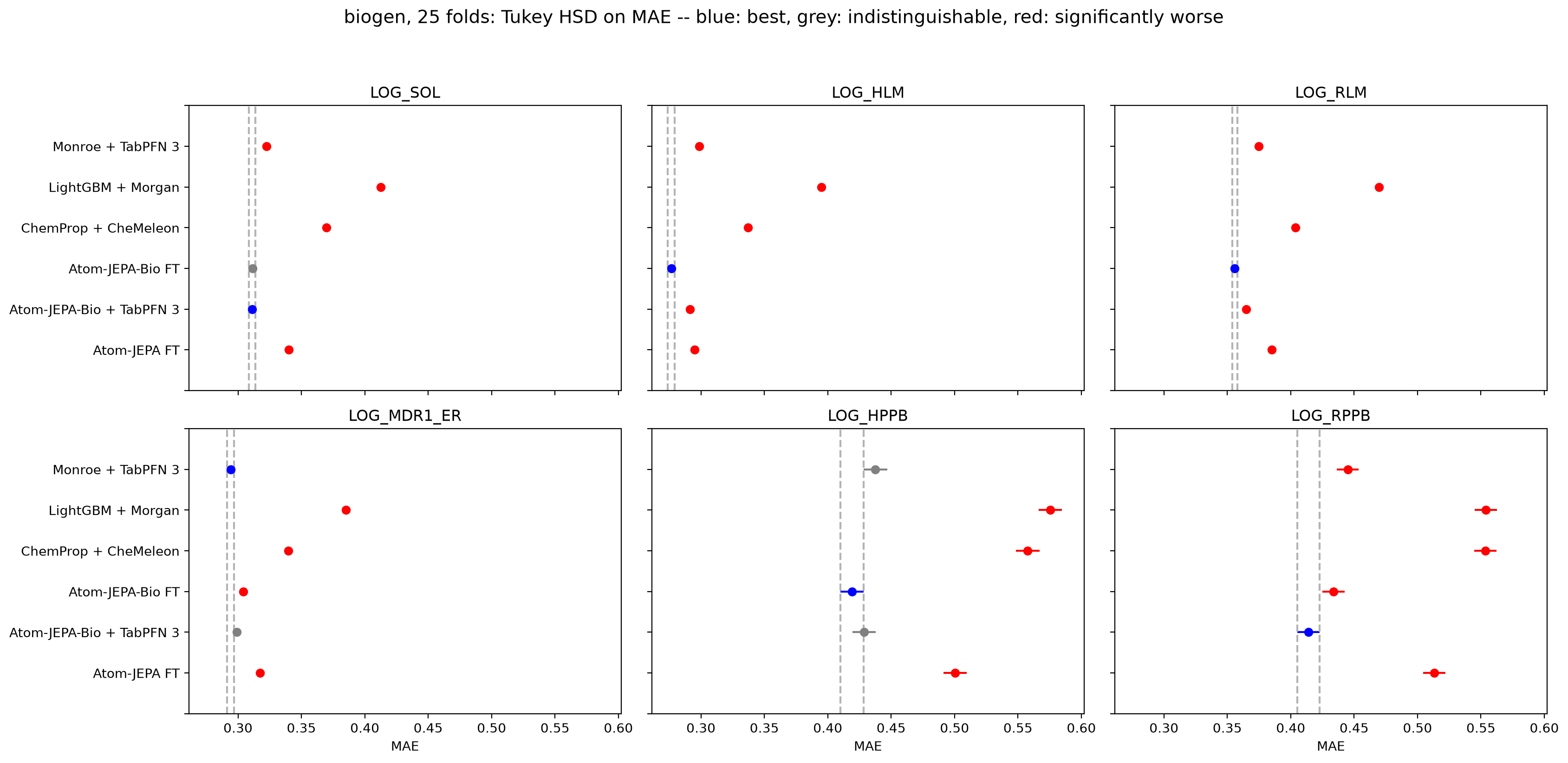
Points show mean MAE over 25 cross-validation folds (5 × 5) with Tukey simultaneous 95% confidence intervals. Blue: best method. Grey: statistically indistinguishable from the best. Red: significantly worse. Dashed lines mark the best method’s interval.
| Endpoint | Atom-JEPA-Bio FT | Atom-JEPA-Bio + TabPFN 3 | Monroe + TabPFN 3 | Atom-JEPA FT | LightGBM + Morgan | ChemProp + CheMeleon |
|---|---|---|---|---|---|---|
| SOL | 0.311 ± 0.007 | 0.311 ± 0.003 | 0.322 ± 0.004 | 0.340 ± 0.006 | 0.413 ± 0.009 | 0.370 ± 0.007 |
| HLM | 0.277 ± 0.012 | 0.291 ± 0.002 | 0.299 ± 0.003 | 0.295 ± 0.008 | 0.395 ± 0.005 | 0.337 ± 0.007 |
| RLM | 0.356 ± 0.007 | 0.365 ± 0.002 | 0.375 ± 0.003 | 0.385 ± 0.005 | 0.470 ± 0.005 | 0.404 ± 0.006 |
| MDR1_ER | 0.304 ± 0.013 | 0.299 ± 0.004 | 0.294 ± 0.002 | 0.317 ± 0.005 | 0.385 ± 0.005 | 0.340 ± 0.004 |
| HPPB | 0.419 ± 0.016 | 0.429 ± 0.019 | 0.438 ± 0.017 | 0.500 ± 0.019 | 0.576 ± 0.033 | 0.558 ± 0.025 |
| RPPB | 0.434 ± 0.020 | 0.414 ± 0.015 | 0.445 ± 0.026 | 0.513 ± 0.023 | 0.554 ± 0.021 | 0.553 ± 0.023 |
Bold: lowest mean. tied: statistically indistinguishable from the best by Tukey HSD (α = 0.05).
ExpansionRx
On ExpansionRx, Atom-JEPA-Bio builds on the original model’s strong ExpansionRx performance, with the clearest gain on LogD, where mean MAE decreases by approximately 9%. Performance remains similar on several other endpoints. Frozen features paired with TabPFN 3 are less successful here than on Biogen ADME. One possible explanation is that the PCBA assays provide more relevant supervision for Biogen ADME than for ExpansionRx. This would suggest that the effectiveness of frozen features, without downstream finetuning, depends on how closely the supervised pretraining tasks align with the downstream task.
TABLE 4
Tukey HSD outcomes on ExpansionRx
| Model | Best alone | Tied for best | Worse | Best or tied |
|---|---|---|---|---|
| Atom-JEPA-Bio FT | 3 | 17 | 7 | 20 / 27 |
| Atom-JEPA FT | 0 | 16 | 11 | 16 / 27 |
| Monroe + TabPFN 3 | 7 | 2 | 18 | 9 / 27 |
| ChemProp + CheMeleon | 0 | 3 | 24 | 3 / 27 |
| Atom-JEPA-Bio + TabPFN 3 | 0 | 0 | 27 | 0 / 27 |
| LightGBM + Morgan | 0 | 0 | 27 | 0 / 27 |
Counted over 27 comparisons (9 endpoints × 3 metrics: MAE, Spearman ρ and R²), each over 25 cross-validation folds (5 × 5). Categories as in Table 2.
FIGURE 2
Test MAE on ExpansionRx with Tukey HSD intervals
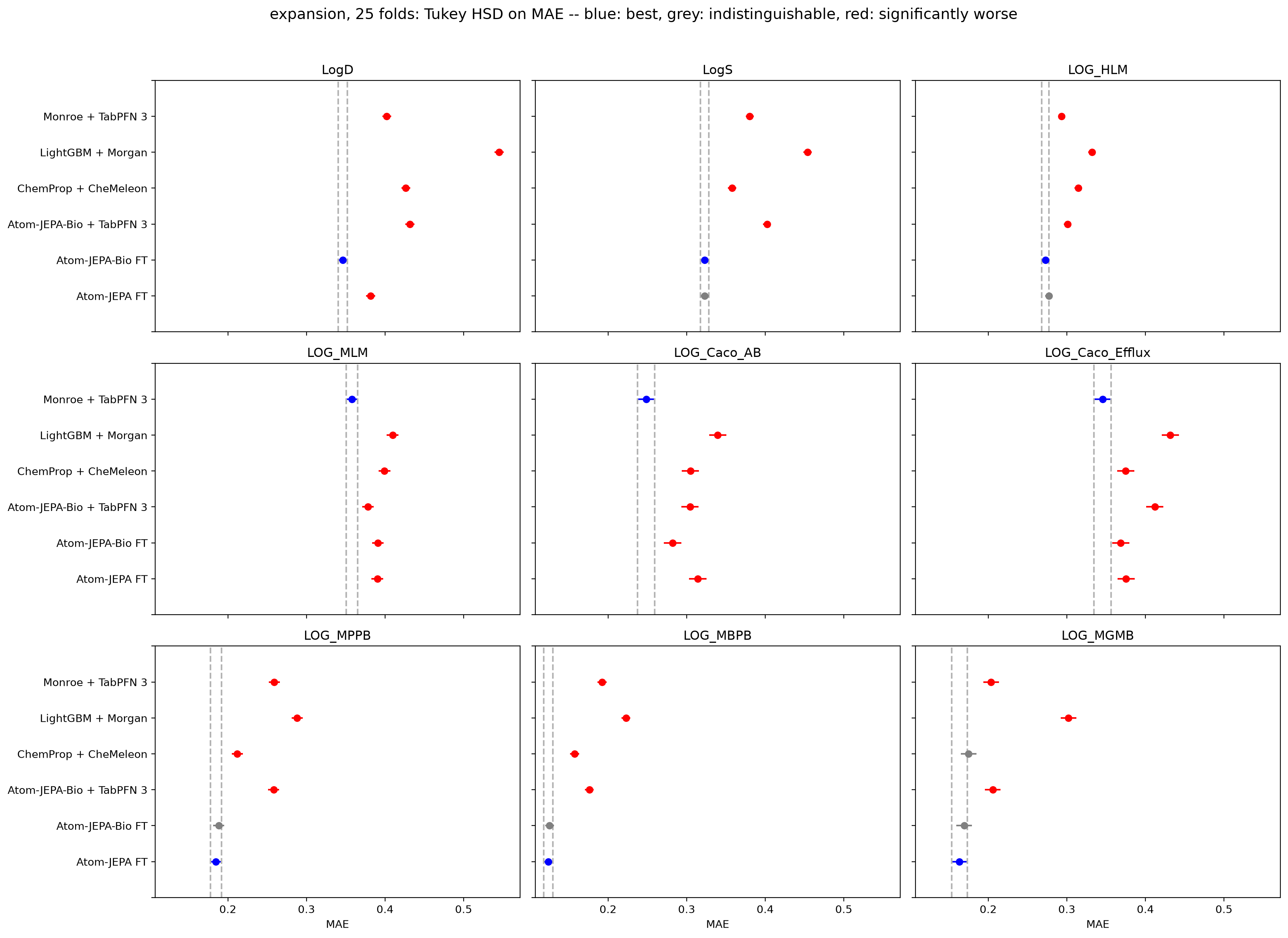
Points show mean MAE over 25 cross-validation folds (5 × 5) with Tukey simultaneous 95% confidence intervals for the nine ExpansionRx endpoints. Blue: best method. Grey: statistically indistinguishable from the best. Red: significantly worse. Dashed lines mark the best method’s interval.
| Endpoint | Atom-JEPA-Bio FT | Atom-JEPA FT | Monroe + TabPFN 3 | Atom-JEPA-Bio + TabPFN 3 | LightGBM + Morgan | ChemProp + CheMeleon |
|---|---|---|---|---|---|---|
| LogD | 0.346 ± 0.014 | 0.382 ± 0.014 | 0.402 ± 0.015 | 0.432 ± 0.011 | 0.545 ± 0.012 | 0.427 ± 0.018 |
| LogS | 0.323 ± 0.011 | 0.323 ± 0.010 | 0.380 ± 0.009 | 0.402 ± 0.012 | 0.454 ± 0.015 | 0.358 ± 0.017 |
| LOG_HLM | 0.273 ± 0.012 | 0.277 ± 0.014 | 0.293 ± 0.009 | 0.301 ± 0.007 | 0.332 ± 0.009 | 0.314 ± 0.014 |
| LOG_MLM | 0.391 ± 0.016 | 0.390 ± 0.017 | 0.358 ± 0.011 | 0.378 ± 0.015 | 0.410 ± 0.014 | 0.399 ± 0.030 |
| LOG_Caco_AB | 0.282 ± 0.033 | 0.314 ± 0.037 | 0.248 ± 0.011 | 0.304 ± 0.017 | 0.340 ± 0.022 | 0.305 ± 0.033 |
| LOG_Caco_Efflux | 0.369 ± 0.036 | 0.375 ± 0.034 | 0.346 ± 0.012 | 0.412 ± 0.015 | 0.432 ± 0.019 | 0.375 ± 0.034 |
| LOG_MPPB | 0.188 ± 0.017 | 0.185 ± 0.018 | 0.259 ± 0.013 | 0.258 ± 0.012 | 0.288 ± 0.020 | 0.212 ± 0.021 |
| LOG_MBPB | 0.126 ± 0.010 | 0.124 ± 0.005 | 0.192 ± 0.016 | 0.176 ± 0.011 | 0.223 ± 0.018 | 0.157 ± 0.018 |
| LOG_MGMB | 0.169 ± 0.014 | 0.163 ± 0.010 | 0.204 ± 0.033 | 0.206 ± 0.028 | 0.302 ± 0.034 | 0.175 ± 0.015 |
Bold: lowest mean. tied: statistically indistinguishable from the best by Tukey HSD (α = 0.05).
Method
As illustrated in Figure 3, Atom-JEPA-Bio extends the original Atom-JEPA framework with a supervised bioassay prediction branch. Overall, this supervised branch is based on adapting the uncertainty-weighted loss used in Monroe. We combine the context encoder’s scalar features with norms of its higher-order features, then apply attention pooling and a linear property head to predict bioassay labels. During second-stage pretraining, this supervised objective (denoted ) is optimized jointly with Atom-JEPA’s original SSL objectives:
We do not add Monroe’s supervised quantum chemistry tasks, conformer denoising, or embedding decorrelation losses. However, we retain Atom-JEPA’s original self-supervised objectives to preserve the strengths of the representations learned in the first pretraining stage. This choice is also supported by our initial small-scale experiments, which indicated better downstream performance when retaining these objectives than when continuing with supervised pretraining alone.
FIGURE 3
Second-stage pretraining of Atom-JEPA-Bio
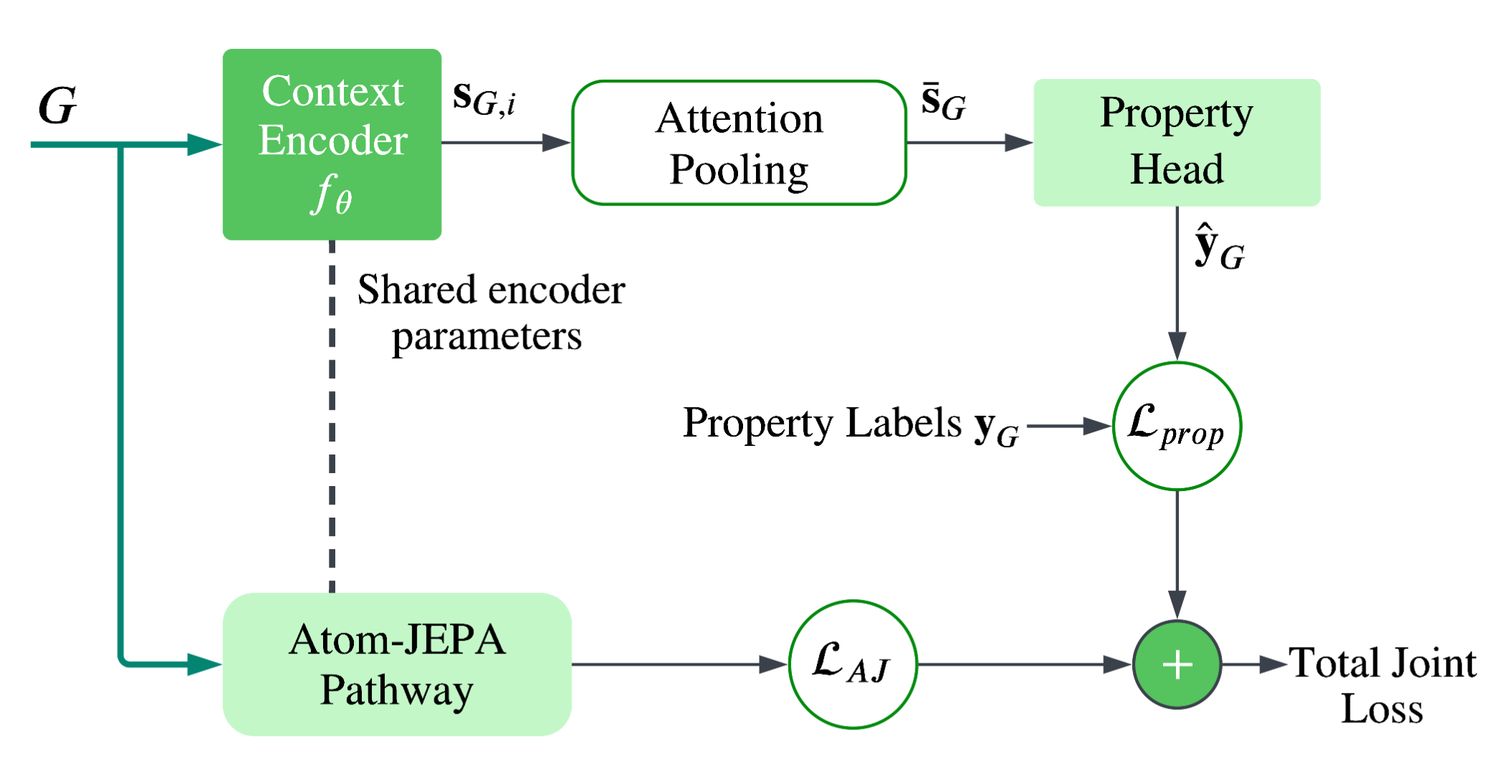
The context encoder is shared with the Atom-JEPA pathway and maps the full 3D molecular input graph to atom-level features . Scalar features and the norms of vector and tensor features are then combined through attention pooling to produce , which the property head maps to bioassay predictions . Training combines uncertainty-weighted supervision on observed assay labels with Atom-JEPA’s original SSL objectives.
PCBA data
The PCBA dataset is a collection of experimental screening data from PubChem BioAssay covering approximately 1.5M molecules and 1.3K bioassays. Each assay defines a binary classification task where molecules are labeled as active or inactive. To match Monroe’s PCBA pretraining data, we follow the same preprocessing and filtering procedure: deduplicating molecules, excluding molecules present in the Polaris or MoleculeACE test sets, and retaining only assays with at least 100 active, 100 inactive, and 1,000 observed training labels. This leaves 1,089 assays.
Supervised objective
First, the context encoder produces atom features from the full 3D input graph :
For each atom , these features consist of scalar, vector, and tensor features, denoted by , , and . Each order has channels. This context encoder is the same one that is used in the Atom-JEPA pathway, and the one that is used after pretraining for downstream tasks.
Attention pooling
We first convert the higher-order features into scalar features by taking their channel-wise norms:
Then we concatenate these norms with the scalar features to construct a -dimensional atom representation:
where denotes concatenation and LN denotes layer normalization. For each attention head , we then compute an atom score and normalize it over the atoms in the graph:
The weighted atom features are then concatenated across heads to obtain the molecule-level representation:
where each head contributes channels, so has dimension .
Property head
Following attention pooling, a linear head followed by a sigmoid produces activity probabilities for the assays:
Here, has shape , and is the predicted probability that molecule is active in assay .
Loss
Following Monroe, we use focal binary cross-entropy loss to address the class imbalance of the label distribution in the PCBA dataset. For an observed label , define the probability assigned to the correct class as
and the class weight as
The loss for assay is averaged over the molecules with observed labels in the batch:
Following Monroe, we learn a log-variance for each assay. Unlike Monroe’s sum over task contributions, we average over only the set of assays with observed labels in the batch:
Larger uncertainty reduces an assay’s weight, while the additive term penalizes excessive uncertainty. Assays without labels in a batch contribute neither a prediction loss nor an uncertainty regularization term, and we mask updates to their log-variance parameters so these remain unchanged for that batch.
Pretraining details and metrics
The encoder and predictor start from the first-stage pretraining run (Atom-JEPA pretraining on the Uni-Mol dataset). The attention pooling and the property head start from randomly initialized weights, which we warm up during an initial freezing period of the encoder.
TABLE 6
Hyperparameters for second-stage pretraining
| Parameter | Value |
|---|---|
| Epochs | 10 (13,640 steps) |
| Batch size | 1,024 (32 GPUs × 32 molecules per GPU) |
| Optimizer | AdamW |
| Peak learning rate | 3.96 × 10⁻⁴ |
| LR schedule | 15% linear warmup, then cosine decay |
| Weight decay | 0.04 |
| Encoder freeze | 1,000 steps |
| EMA momentum τ | 0.998 → 1.0 |
| 1 | |
| 10 | |
| Focal loss α | 0.25 |
| Focal loss γ | 2 |
Balancing and
To understand how the Atom-JEPA and supervised objectives interact during second-stage pretraining, we looked at what each loss does to the context encoder: every 200 steps we compute the gradient of each weighted term with respect to the context encoder’s parameters, and compare their sizes and directions.
With and (denoted AJ for short), the property gradient starts at roughly 0.4× the size of the Atom-JEPA gradient (Figure 4, left). So early on it adds a meaningful signal without overriding the Atom-JEPA objective. As training progresses, the Atom-JEPA loss converges and shrinks about threefold, while the property gradient stays roughly constant, which results in about equal pull on the encoder around epoch 8 and around 2× by the end.
While interpreting the gradient directions is less clear-cut, their cosine similarity suggests that the supervised signal pushes the context encoder in largely new directions rather than undoing what the Atom-JEPA objectives learn (Figure 4, right). However, despite an overall median of 0.1, the measurements are noisy and show periods of both positive and negative alignment, so we view this as an indication rather than a firm conclusion.
Overall, these diagnostics suggest a reasonable balance between the two objectives. That said, we can’t establish for certain that it is an optimal choice. Whether different weights could improve downstream performance remains an open question.
FIGURE 4
Gradient balance on the context encoder
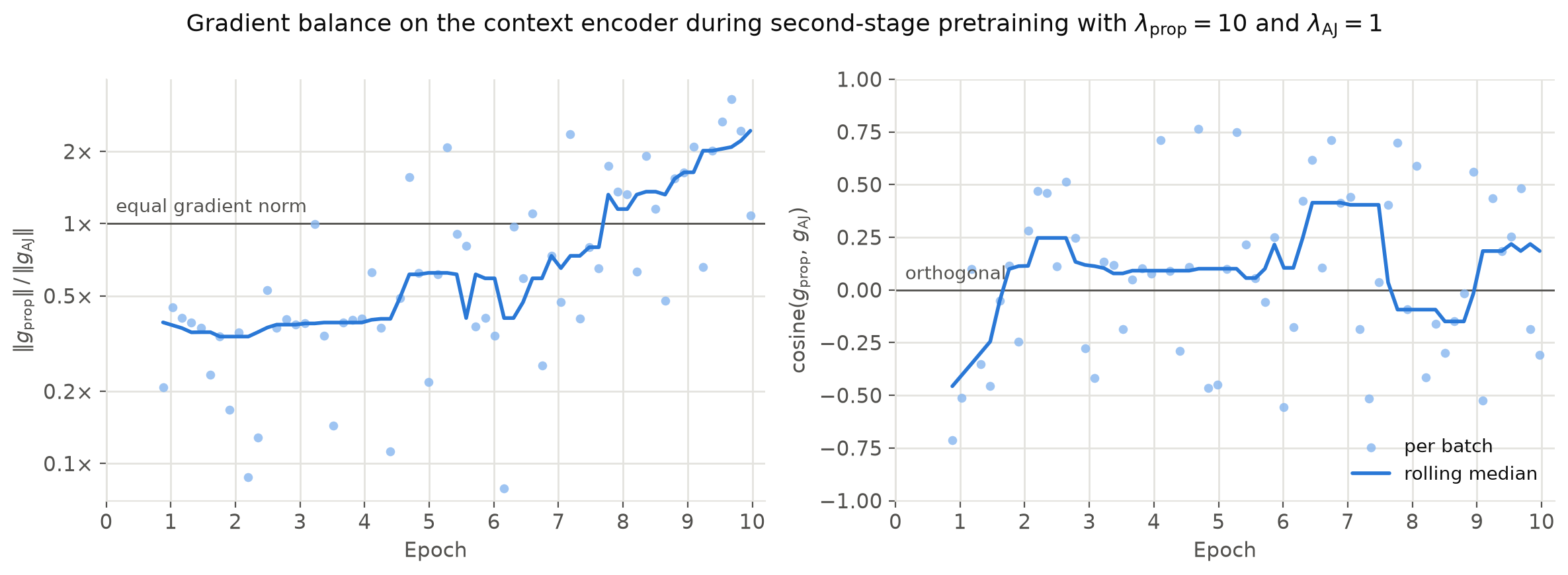
Second-stage pretraining with and . Left: size of the property gradient relative to the Atom-JEPA gradient, on a log scale. Right: cosine similarity between the two gradients. Dots are individual measurements every 200 steps; the line is a rolling median. Measurements begin after the 1,000-step encoder freeze.
Representation collapse metrics
As in the original Atom-JEPA paper, we watch for representation collapse during pretraining using the target encoder’s pooled molecule embeddings. Every 200 steps we stack the embeddings from all GPUs into one matrix and compute the RankMe and α-ReQ metrics. RankMe measures how many of the 256 embedding dimensions are effectively in use, i.e. a value going towards 1 means collapse. α-ReQ measures how quickly variance decays across those dimensions; a large value means a few directions dominate, and a moderate value is healthy.
In the first pretraining stage, RankMe plateaued around 80 and α-ReQ settled in a moderate range. The second stage keeps it that way: RankMe rises from 93 to 119, and α-ReQ stays roughly flat (1.74 → 1.69). So adding the property objective spreads information over more dimensions instead of collapsing the representations.
FIGURE 5
RankMe and α-ReQ during second-stage pretraining
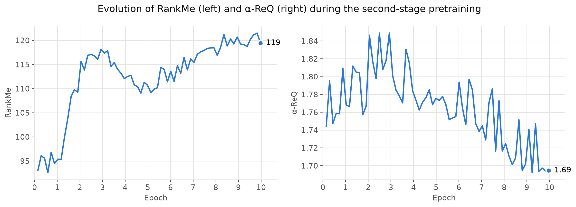
RankMe (left) and α-ReQ (right) of the target encoder’s pooled embeddings during second-stage pretraining.
Looking ahead
Atom-JEPA-Bio gives us an encouraging first step toward combining the scale of Atom-JEPA’s self-supervised learning with the information in experimental labels. We’re excited to continue building on Atom-JEPA and Atom-JEPA-Bio, exploring how larger and more diverse datasets of both labeled and unlabeled atomistic systems can help us learn more general representations. These results suggest there is more to gain from combining the two sources of information, and we look forward to investigating how far this approach can take us.
Get the model on Hugging FaceBrowse the codeBack to the Atom-JEPA project page
References
- Atom-JEPA: Petersen et al. (2026). Atom-JEPA: Joint-Embedding Predictive Architecture for 3D Atomistic Systems.
- Uni-Mol: Zhou et al. (2023). Uni-Mol: A Universal 3D Molecular Representation Learning Framework.
- Monroe: Banaszewski and Fitzgibbon (2026). Monroe: A Molecular Foundation Model for In-Context Probabilistic Inference.
- PCBA pretraining dataset: Graphium (2024). PCBA-1328-1564k-v1.
- Biogen ADME: Fang et al. (2023). Prospective Validation of Machine Learning Algorithms for Absorption, Distribution, Metabolism, and Excretion Prediction: An Industrial Perspective.
- ExpansionRx: OpenADMET and Expansion Therapeutics (2026). OpenADMET–ExpansionRx Blind Challenge Data.
- TabPFN 3: Grinsztajn et al. (2026). TabPFN-3: Technical Report.
- CheMeleon: Burns et al. (2026). Deep Learning Foundation Models for Low-Data Regimes from Classical Molecular Descriptors.
- Chemprop: Graff et al. (2026). Chemprop v2: An Efficient, Modular Machine Learning Package for Chemical Property Prediction.
- LightGBM: Ke et al. (2017). LightGBM: A Highly Efficient Gradient Boosting Decision Tree.
- Morgan/ECFP fingerprints: Rogers and Hahn (2010). Extended-Connectivity Fingerprints.
- RankMe: Garrido et al. (2023). RankMe: Assessing the Downstream Performance of Pretrained Self-Supervised Representations by Their Rank.
- α-ReQ: Agrawal et al. (2022). α-ReQ: Assessing Representation Quality in Self-Supervised Learning by Measuring Eigenspectrum Decay.